42 pivot table row labels format

Formatting Row Labels in Pivot Table/Chart I want the pivot chart to match the 'simple' chart in look and feel. Any attempts to change the formatting of the row labels to 'h' is promptly ignored by Excel. Note the two tasks that occur at hour 18 (one at 18:00 and the other at 18:20 (you will need to see the formatting to truly see the minutes)). Repeat item labels in a PivotTable Right-click the row or column label you want to repeat, and click Field Settings. Click the Layout & Print tab, and check the Repeat item labels box. Make sure Show item labels in tabular form is selected. Notes: When you edit any of the repeated labels, the changes you make are applied to all other cells with the same label.

Quick tip: Rename headers in pivot table so they are ... 15.03.2018 · Change the order of pivot table row labels; First and last date of a sale with pivots; Introduction to pivot tables; Pivots from multiple tables; What is your favorite pivot tip? Please share in comments. Share on facebook. Facebook Share on twitter. Twitter Share on linkedin. LinkedIn Share this tip with your colleagues Get FREE Excel + Power BI Tips. Simple, fun and …

Pivot table row labels format

How to Select Parts of Excel Pivot Table 12.07.2021 · Select a cell in the pivot table, and on the Ribbon, click the Options tab. In the Actions group, click Select; Click Entire PivotTable. Move a Pivot Table. Instead of manually selecting a large pivot table and moving it, you can use a built-in command to move a pivot table. Watch this short video to see the steps, and the written instructions ... Excel Pivot Table - Format Numbers in Rows To format rows or columns in a PT, hover the mouse at the top of the column or beginning of the row until a black arrow appears, click to highlight the row/column and format as usual. For Display labels from next field in same column, uncheck this, follow above procedure, then recheck. Paula Scharf Automatic Row And Column Pivot Table Labels Select the data set you want to use for your table The first thing to do is put your cursor somewhere in your data list Select the Insert Tab Hit Pivot Table icon Next select Pivot Table option Select a table or range option Select to put your Table on a New Worksheet or on the current one, for this tutorial select the first option Click Ok

Pivot table row labels format. Pivot Table Row Labels In the Same Line - Beat Excel! After creating a pivot table in Excel, you will see the row labels are listed in only one column. But, if you need to put the row labels on the same line to view the data more intuitively and clearly as following screenshots shown. Pivot Table Conditional Formatting for Different Rows ... Hello, It is possible! All you have to do: Select Your Pivot Table and: Go to Conditional Formatting -> New Rule -> Choose All cells showing "duration" values for "Type and "Date Selection" under "Apply Rule To" section -> Use a Formula to Determine which cells to format and enter the following formula: =AND(A6="Cars",A6>3), You can create new rules for other two conditions as well: Pivot table row labels side by side - Excel Tutorials You can copy the following table and paste it into your worksheet as Match Destination Formatting. Now, let's create a pivot table ( Insert >> Tables >> Pivot Table) and check all the values in Pivot Table Fields. Fields should look like this. Right-click inside a pivot table and choose PivotTable Options…. Check data as shown on the image below. Formatting Tips for Pivot Tables - Goodly Right Click on the Pivot and go to Pivot Table Options Under Layout & Format Tab --> For empty cells show: "NIL" (you can customize this) Tip #11 Custom Sorting of Row / Column values This happens a lot. The default sorting order of row or column (text) labels is A-Z or Z-A. Now there are 2 ways to sort the values in a custom order

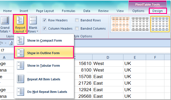
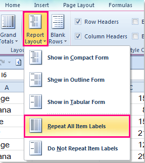
Excel Pivot Table Row labels - Stack Overflow Right click on the pivot, go to PivotTable Options, Display Tab. Click on "Classic Pivot Table Layout" Go to each field (column), right click, field settings, layout & print tab. Click on "Repeat Item Labels" That should give you the table you're looking for. Format Pivot Table Labels Based on Date Range - Excel ... In the pivot table, remove any filters that have been applied - all the rows need to be visible before you apply the conditional formatting. Select all the dates in the Row Labels that you want to format. On the Ribbon, click the Home tab, and then in the Styles group, click Conditional Formatting. Design the layout and format of a PivotTable In the PivotTable Options dialog box, click the Layout & Format tab, and then under Layout, select or clear the Merge and center cells with labels check box. Note: You cannot use the Merge Cells check box under the Alignment tab in a PivotTable. Change the display of blank cells, blank lines, and errors Change Pivot Table Layout using VBA - Access-Excel.Tips Since "Row Labels" refer to both Department and Empl ID as they display in one column, it uses a generic name "Row Labels". Excel 2007 and onwards - Outline layout There is another new layout called "Outline", where the layout format is between "Tabular" and "Compact".

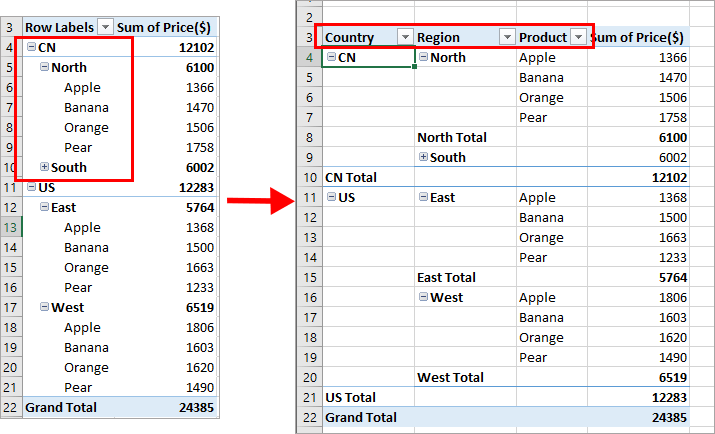
Automate Pivot Table with Python (Create, Filter and ... 22.05.2021 · Photo by Jasmine Huang on Unsplash. In Automate Excel with Python, the concepts of the Excel Object Model which contain Objects, Properties, Methods and Events are shared.The tricks to access the Objects, Properties, and Methods in Excel with Python pywin32 library are also explained with examples.. Now, let us leverage the automation of Excel report … Conditional formatting in pivot tables using rows ... I have a simple pivot that splits the data across rows based on ranges, e.g. 600-650, 550-600 etc. I want to tell Excel to use a specific fill color for any cell on the same row as a specific row label, so for example if the row label value is "600-650" the data cells on the table will be filled in yellow etc. How to repeat row labels for group in pivot table? In Excel, when you create a pivot table, the row labels are displayed as a compact layout, all the headings are listed in one column. Sometimes, you need to convert the compact layout to outline form to make the table more clearly. But in tphe outline layout, the headings will be displayed at the top of the group. Overwrite pivot table conditional format based on row label As far as I know, using the one rule in the Conditional formatting, we can only format the cells with one color if the condition is true and if the same condition is false, the formatting of the cell will be blank and if both conditions are true, the formatting of cell depends on the highest ranking/priority of the rules in Conditional formatting.

56 DOWNLOAD PRINTABLE PIVOT TABLE X AND Y AXIS PDF DOC ZIP - Pivot

Changing Blank Row Labels - Excel Pivot Tables You can manually change the (blank) labels in the Row or Column Labels areas by typing over them in the pivot table. You can type any text to replace the (Blank) entry, but you can't clear the cell and leave it empty: Select one of the Row or Column Labels that contains the text (blank). Type N/A in the cell, and then press the Enter key.

How to repeat row labels for group in pivot table?

How do I add formatting to a pivot table(i.e., borders ... I have been trying for months to figure out how to apply formatting such as borders and colors to a pivot table. I spend hours adjusting and tweaking the formatting of the pivot table so it looks just like it needs to, but as soon as the worksheet is refreshed to update the pivot table data - all my formatting work is lost.

32 Pivot Table Blank Row Label - Labels For You

How to remove bold font of pivot table in Excel? After creating a pivot table in a worksheet, you will see the font of row labels, subtotal rows and Grand Total rows are bold. If you want to un-bold these rows, the first consider is to apply the Bold feature to remove the bold font. But, in pivot table, you will find this feature will not work normally. Today, I will talk about how to quickly ...

Pivot Table Excel 2007 Repeat Row Labels | Elcho Table

How to Customize Your Excel Pivot Chart Data Labels - dummies To add data labels, just select the command that corresponds to the location you want. To remove the labels, select the None command. If you want to specify what Excel should use for the data label, choose the More Data Labels Options command from the Data Labels menu. Excel displays the Format Data Labels pane.

33 Pivot Table Blank Row Label - Labels Database 2020

How to Format Excel Pivot Table - Contextures Excel Tips Select a cell in the pivot table, and on the Ribbon, click the Design tab. In the PivotTable Styles gallery, right-click the style you want to duplicate. In the context menu, click Duplicate. Next, follow the steps in the Modify the PivotTable Style section (below), to name and modify the new style. TOP.

Creating Excel pivot tables ‒ Qlik NPrinting

Conditional Formatting on Pivot Table row labels In srcFromPowerPivot sheet cell A is from powerpivot under row label comparing the dates in cell C (3 dates) and the condtional formatting doesnt work. In cell J it worked cos I dragged under value instead of row label. In the srcFromWorksheet it worked even though it is under rowlabel. Sheet3 is just a copy of powerpivot data.

Repeat Pivot Table row labels • AuditExcel.co.za Pivot Tables Course

Excel Pivot Table Row Label Column Display Format Excel Pivot Table Row Label Column Display Format . ... column or filter in Pivot Table. But the format in which it is showing is not right. Eg, It is showing like 200,911. instead i want to remove comma, and show row or column as . 200911. I tried some steps to modify format, but didn't get any solution. ...

How to Setup Source Data for Pivot Tables - Unpivot in Excel

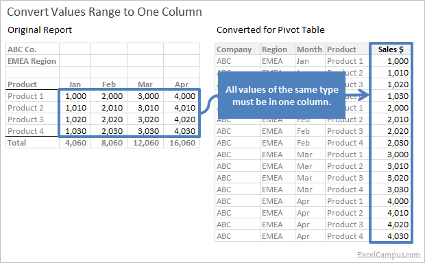
101 Advanced Pivot Table Tips And Tricks ... - How To Excel 25.04.2022 · When using a pivot table your source data will need to be in a tabular format. This means your data is in a table with rows and columns. The first row should contain your column headings which describes the data directly below in that column. There should be no blank column headings in your data. Each row after the column headings should pertain to exactly …

31 How To Label Excel Columns - Labels Database 2020

Excel Pivot Table Macro Paste Format Values 10.07.2021 · Copy Pivot Table Format - Manual. To manually copy pivot table values and formatting, use one of the techniques shown below. If your pivot table does NOT have any fields in the Filters area, use method 1 or 3. For pivot tables with report filters, use method 2 or 3. Manual steps - no report filters; Manual steps - with report filters

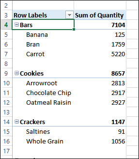
Better Format for Pivot Table Headings – Excel Pivot Tables

Remove row labels from pivot table - AuditExcel.co.za Click on the Pivot table Click on the Design tab Click on the report layout button Choose either the Outline Format or the Tabular format If you like the Compact Form but want to remove 'row labels' from the Pivot Table you can also achieve it by Clicking on the Pivot Table Clicking on the Analyse tab

Components | CLEARIFY

Formatting Pivot Table Row Labels by Level | MrExcel ... hover your cursor over the top line of one of the SubTotals of the Level that you want to format until you get a downward pointing, then left click - that should highlight all the cells at that level right click while hovering over one of the selected cells to format it OR hit Ctrl+F1

Pivot table row labels in separate columns • AuditExcel.co.za

How to Apply Conditional Formatting in Pivot Table? (with ... Step 3: And drag down Product in Row label and months in the value fields. The pivot table looks like this, Step 4: Now, our motive is to highlight those cells which have the highest number of product sold in each row. Select any cell in the pivot table. Click on Conditional formatting and click on a new rule. Step 5: In the first option, apply ...

Excel KPI Dashboard to Monitor Salesman

How to make row labels on same line in pivot table? Make row labels on same line with PivotTable Options You can also go to the PivotTable Options dialog box to set an option to finish this operation. 1. Click any one cell in the pivot table, and right click to choose PivotTable Options, see screenshot: 2.

How to Sort Pivot Table Row Labels, Column Field Labels and Data Values with Excel VBA Macro ...

How to rename group or row labels in Excel PivotTable? To rename Row Labels, you need to go to the Active Field textbox. 1. Click at the PivotTable, then click Analyze tab and go to the Active Field textbox. 2. Now in the Active Field textbox, the active field name is displayed, you can change it in the textbox.

Share :