40 excel chart horizontal axis labels
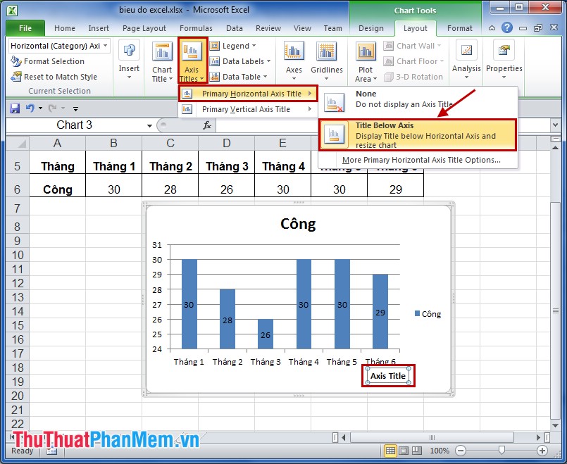
How to add axis label to chart in Excel? - ExtendOffice You can insert the horizontal axis label by clicking Primary Horizontal Axis Title under the Axis Title drop down, then click Title Below Axis, and a text box will appear at the bottom of the chart, then you can edit and input your title as following screenshots shown. 4. How to display text labels in the X-axis of scatter chart in Excel? Display text labels in X-axis of scatter chart Actually, there is no way that can display text labels in the X-axis of scatter chart in Excel, but we can create a line chart and make it look like a scatter chart. 1. Select the data you use, and click Insert > Insert Line & Area Chart > Line with Markers to select a line chart. See screenshot: 2.
Adjusting the Angle of Axis Labels (Microsoft Excel) Right-click the axis labels whose angle you want to adjust. Excel displays a Context menu. Click the Format Axis option. Excel displays the Format Axis task pane at the right side of the screen. Click the Text Options link in the task pane. Excel changes the tools that appear just below the link. Click the Textbox tool.

Excel chart horizontal axis labels
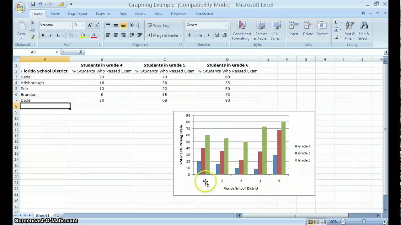
How to Change Horizontal Axis Values - Excel & Google Sheets Similar to what we did in Excel, we can do the same in Google Sheets. We'll start with the date on the X Axis and show how to change those values. Right click on the graph. Select Data Range. 3. Click on the box under X-Axis. 4. Click on the Box to Select a data range. 5. Two-Level Axis Labels (Microsoft Excel) Excel automatically recognizes that you have two rows being used for the X-axis labels, and formats the chart correctly. (See Figure 1.) Since the X-axis labels appear beneath the chart data, the order of the label rows is reversed—exactly as mentioned at the first of this tip. Figure 1. Two-level axis labels are created automatically by Excel. Change axis labels in a chart - support.microsoft.com Right-click the category labels you want to change, and click Select Data. In the Horizontal (Category) Axis Labels box, click Edit. In the Axis label range box, enter the labels you want to use, separated by commas. For example, type Quarter 1,Quarter 2,Quarter 3,Quarter 4. Change the format of text and numbers in labels
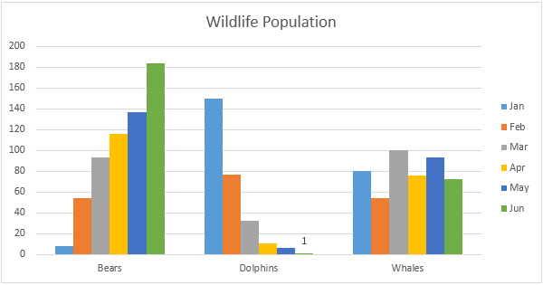
Excel chart horizontal axis labels. Excel charts: add title, customize chart axis, legend and data labels ... Click anywhere within your Excel chart, then click the Chart Elements button and check the Axis Titles box. If you want to display the title only for one axis, either horizontal or vertical, click the arrow next to Axis Titles and clear one of the boxes: Click the axis title box on the chart, and type the text. How-to Highlight Specific Horizontal Axis Labels in Excel Line Charts ... In this video, you will learn how to highlight categories in your horizontal axis for an Excel chart. This is in answer to "I am trying to bold 5 months (ou... Move Horizontal Axis to Bottom - Excel & Google Sheets Moving X Axis to the Bottom of the Graph. Click on the X Axis; Select Format Axis . 3. Under Format Axis, Select Labels. 4. In the box next to Label Position, switch it to Low. Final Graph in Excel. Now your X Axis Labels are showing at the bottom of the graph instead of in the middle, making it easier to see the labels. How to wrap X axis labels in a chart in Excel? - ExtendOffice And you can do as follows: 1. Double click a label cell, and put the cursor at the place where you will break the label. 2. Add a hard return or carriages with pressing the Alt + Enter keys simultaneously. 3. Add hard returns to other label cells which you want the labels wrapped in the chart axis.
Excel tutorial: How to create a multi level axis To straighten out the labels, I need to restructure the data. First, I'll sort by region and then by activity. Next, I'll remove the extra, unneeded entries from the region column. The goal is to create an outline that reflects what you want to see in the axis labels. Now you can see we have a multi level category axis. Excel tutorial: How to customize axis labels Instead you'll need to open up the Select Data window. Here you'll see the horizontal axis labels listed on the right. Click the edit button to access the label range. It's not obvious, but you can type arbitrary labels separated with commas in this field. So I can just enter A through F. When I click OK, the chart is updated. Excel Chart: Horizontal Axis Labels won't update I created the data set in Excel 2016, selected the data and inserted a line chart. I sent one line to the secondary axis. The X axis still shows the correct labels. I sent the other line to the secondary axis and brought the first line back to the primary axis. The X axis labels are still correct. In short, I cannot reproduce the problem. Excel not showing all horizontal axis labels [SOLVED] 1) The horizontal category axis data range was row 3 to row 34, just as you indicated. 2) The range for the Mean Temperature series was row 4 to row 34. I assume you intended this to be the same rows as the horizontal axis data, so I changed it to row3 to row 34. The final 1 immediately appeared.
Change axis labels in a chart in Office - support.microsoft.com In charts, axis labels are shown below the horizontal (also known as category) axis, next to the vertical (also known as value) axis, and, in a 3-D chart, next to the depth axis. The chart uses text from your source data for axis labels. To change the label, you can change the text in the source data. Text Labels on a Horizontal Bar Chart in Excel - Peltier Tech On the Excel 2007 Chart Tools > Layout tab, click Axes, then Secondary Horizontal Axis, then Show Left to Right Axis. Now the chart has four axes. We want the Rating labels at the bottom of the chart, and we'll place the numerical axis at the top before we hide it. In turn, select the left and right vertical axes. Change the scale of the horizontal (category) axis in a chart The horizontal (category) axis, also known as the x axis, of a chart displays text labels instead of numeric intervals and provides fewer scaling options than are available for a vertical (value) axis, also known as the y axis, of the chart. However, you can specify the following axis options: Interval between tick marks and labels How to group (two-level) axis labels in a chart in Excel? (1) In Excel 2007 and 2010, clicking the PivotTable > PivotChart in the Tables group on the Insert Tab; (2) In Excel 2013, clicking the Pivot Chart > Pivot Chart in the Charts group on the Insert tab. 2. In the opening dialog box, check the Existing worksheet option, and then select a cell in current worksheet, and click the OK button. 3.
Excel Chart, Select Data Source, Select All Horizontal Axis Labels - Stack Overflow
How to Insert Axis Labels In An Excel Chart | Excelchat How to add horizontal axis labels in Excel 2016/2013 We have a sample chart as shown below Figure 2 - Adding Excel axis labels Next, we will click on the chart to turn on the Chart Design tab We will go to Chart Design and select Add Chart Element Figure 3 - How to label axes in Excel
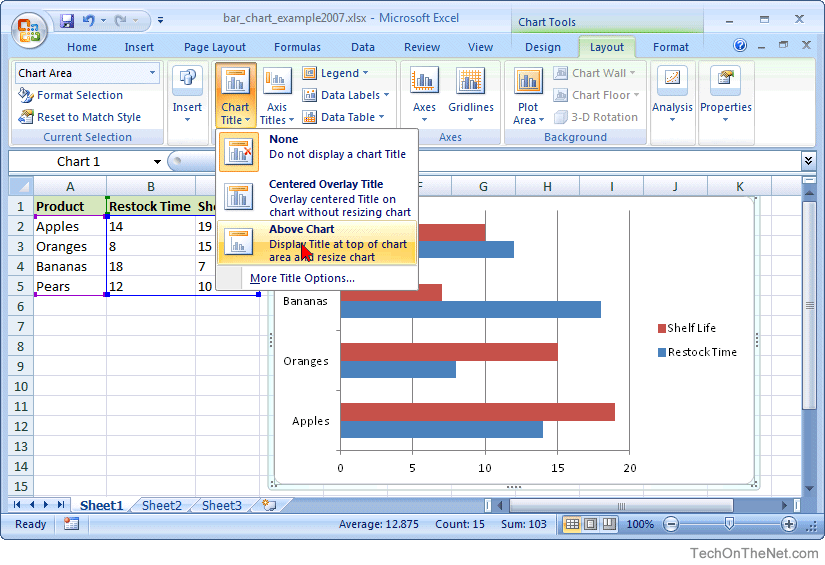
MS Excel 2007: How to Create a Bar Chart
How to rotate axis labels in chart in Excel? - ExtendOffice Rotate axis labels in chart of Excel 2013 If you are using Microsoft Excel 2013, you can rotate the axis labels with following steps: 1. Go to the chart and right click its axis labels you will rotate, and select the Format Axis from the context menu. 2.
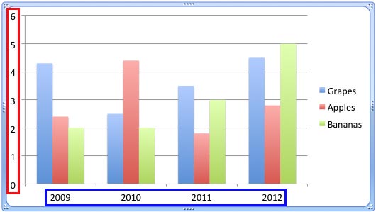
Add Horizontal Category Axis Label Excel
How to create two horizontal axes on the same side 2. Select the data series which you want to see using the secondary horizontal axis. 3. On the Chart Design tab, in the Chart Layouts group, click the Add Chart Element drop-down list: Choose the Axes list and then click Secondary Horizontal: Excel adds the secondary horizontal axis for the selected data series (on the top of the plot area):
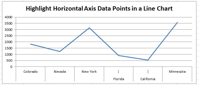
30 How To Label Points In Excel - Labels For You
How to add second horizontal axis labels to Excel chart Jul 20, 2017. #2. Just create a vertical label and then move it where you want. Then click on the chart and hit chart format. Click on the label, go to alignment in the chart format, and change text direction. J.
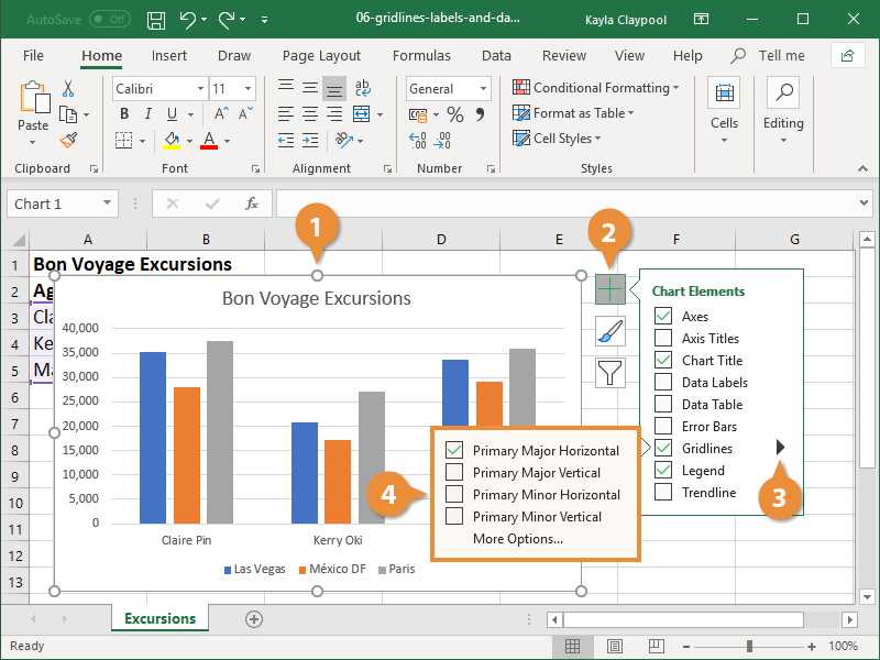
34 Excel Chart Label Axis - Labels 2021
How To Add Axis Labels In Excel [Step-By-Step Tutorial] First off, you have to click the chart and click the plus (+) icon on the upper-right side. Then, check the tickbox for 'Axis Titles'. If you would only like to add a title/label for one axis (horizontal or vertical), click the right arrow beside 'Axis Titles' and select which axis you would like to add a title/label. Editing the Axis Titles
Charts in Excel - Easy Excel Tutorial
Change axis labels in a chart - support.microsoft.com Right-click the category labels you want to change, and click Select Data. In the Horizontal (Category) Axis Labels box, click Edit. In the Axis label range box, enter the labels you want to use, separated by commas. For example, type Quarter 1,Quarter 2,Quarter 3,Quarter 4. Change the format of text and numbers in labels
Link chart title to cell
Two-Level Axis Labels (Microsoft Excel) Excel automatically recognizes that you have two rows being used for the X-axis labels, and formats the chart correctly. (See Figure 1.) Since the X-axis labels appear beneath the chart data, the order of the label rows is reversed—exactly as mentioned at the first of this tip. Figure 1. Two-level axis labels are created automatically by Excel.

How to change horizontal axis labels in Excel 2021, geef een boeiende presentatie
How to Change Horizontal Axis Values - Excel & Google Sheets Similar to what we did in Excel, we can do the same in Google Sheets. We'll start with the date on the X Axis and show how to change those values. Right click on the graph. Select Data Range. 3. Click on the box under X-Axis. 4. Click on the Box to Select a data range. 5.
How to Change X axis Categories - YouTube

How to make a horizontal bar chart in excel - MISHKANET.COM

Excel Custom Chart Labels • My Online Training Hub

How to Change Horizontal Axis Labels in Excel 2010 - Solve Your Tech
Cách vẽ biểu đồ trong Excel
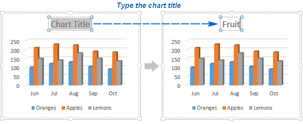
34 Excel Graph Add Axis Label - Labels Database 2020

Column Chart in Excel - EASY Excel Tutorial
Excel Horizontal (Category) Axis Labels for all graphs - Microsoft Community
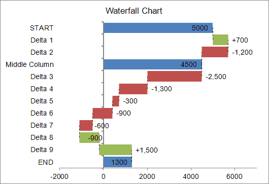
Waterfall Chart Template for Excel
Post a Comment for "40 excel chart horizontal axis labels"