45 how to add two data labels in excel pie chart
Excel charts: add title, customize chart axis, legend and data labels Click anywhere within your Excel chart, then click the Chart Elements button and check the Axis Titles box. If you want to display the title only for one axis, either horizontal or vertical, click the arrow next to Axis Titles and clear one of the boxes: Click the axis title box on the chart, and type the text. How to Make a 2010 Excel Pie Chart with Labels Both Inside and Outside ... Harassment is any behavior intended to disturb or upset a person or group of people. Threats include any threat of suicide, violence, or harm to another.
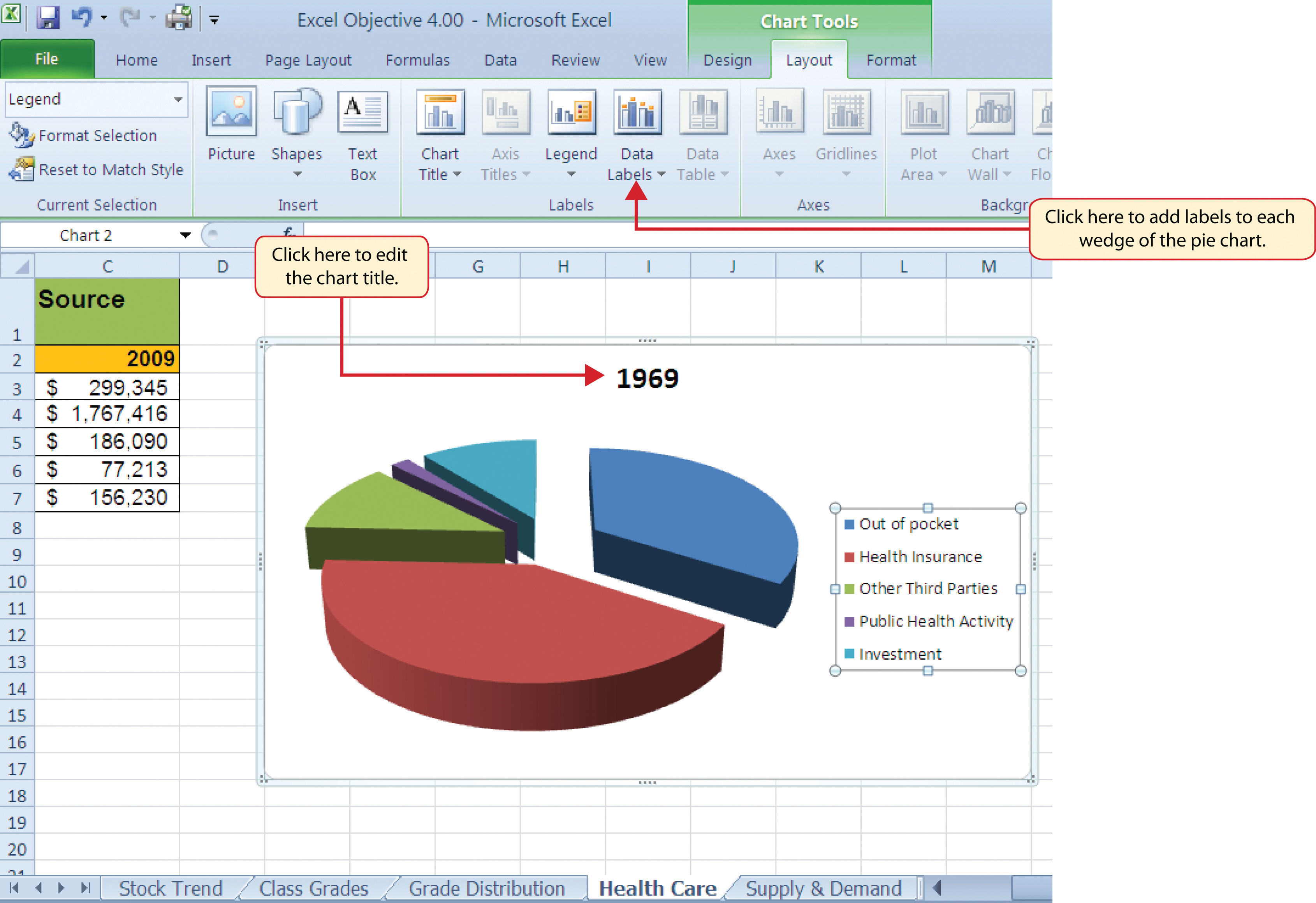
How to Add Data Labels in Excel - Excelchat | Excelchat After inserting a chart in Excel 2010 and earlier versions we need to do the followings to add data labels to the chart; Click inside the chart area to display the Chart Tools. Figure 2. Chart Tools. Click on Layout tab of the Chart Tools. In Labels group, click on Data Labels and select the position to add labels to the chart.

How to add two data labels in excel pie chart
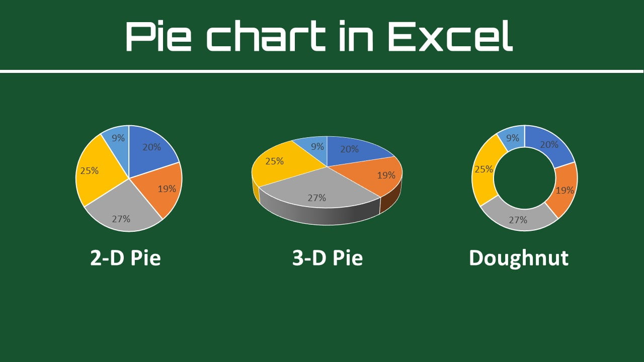
Multiple Data Labels on a Pie Chart | MrExcel Message Board So I have a table with 8 rows and 3 columns. This table includes: Column 1 - shipment name Column 2 - shipment cost Column 3 - shipment weight I have created a pie chart from this table, which covers the first two columns. Displayed next to each slice is a label with the shipment name, shipment cost, and percent share of the pie. Excel Pie Chart - How to Create & Customize? (Top 5 Types) Select the cell range A1:B7 > go to the " Insert " tab > go to the " Charts " group > click on the " Insert Pie or Doughnut Chart " drop-down > click the " Pie " type in the " 2-D Pie " option, as shown below. #Adding Data Labels We will customize the Pie Chart in Excel by Adding Data Labels. Create two data labels in pie chart? | MrExcel Message Board You have already figured out how to add an image that fills the sector of the pie chart but as far as I know you cannot add an icon or image over the actual pie chart sector, in such a way that it adjusts with the values. If you add it as a static image next to the legend, at least the legend does not move when the values change. Cheers.
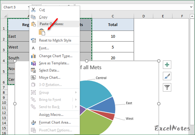
How to add two data labels in excel pie chart. How to Add Data Labels to an Excel 2010 Chart - dummies Use the following steps to add data labels to series in a chart: Click anywhere on the chart that you want to modify. On the Chart Tools Layout tab, click the Data Labels button in the Labels group. None: The default choice; it means you don't want to display data labels. Center to position the data labels in the middle of each data point. How to Combine or Group Pie Charts in Microsoft Excel Combine Pie Chart into a Single Figure. Another reason that you may want to combine the pie charts is so that you can move and resize them as one. Click on the first chart and then hold the Ctrl key as you click on each of the other charts to select them all. Click Format > Group > Group. All pie charts are now combined as one figure. How to add or move data labels in Excel chart? - ExtendOffice To add or move data labels in a chart, you can do as below steps: In Excel 2013 or 2016 1. Click the chart to show the Chart Elements button . 2. Then click the Chart Elements, and check Data Labels, then you can click the arrow to choose an option about the data labels in the sub menu. See screenshot: In Excel 2010 or 2007 c# - Add data labels to excel pie chart - Stack Overflow 1. Very awesome! Thanks! I originally tried series.ApplyDataLabels (blahblah); except I put it before filling in the data, and that's probably why it didn't work. Also, the xRange and yRange stuff were part of an incomplete refactor. Thanks for catching that :P.
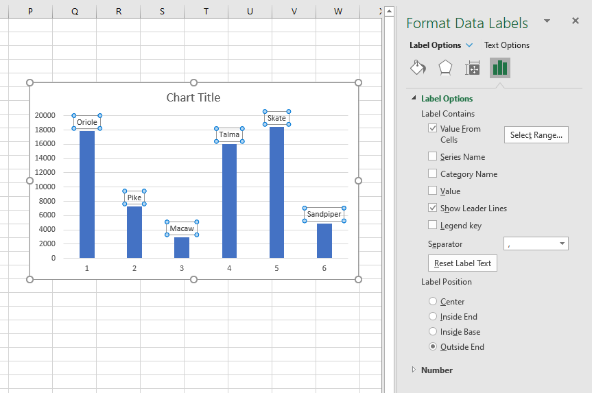
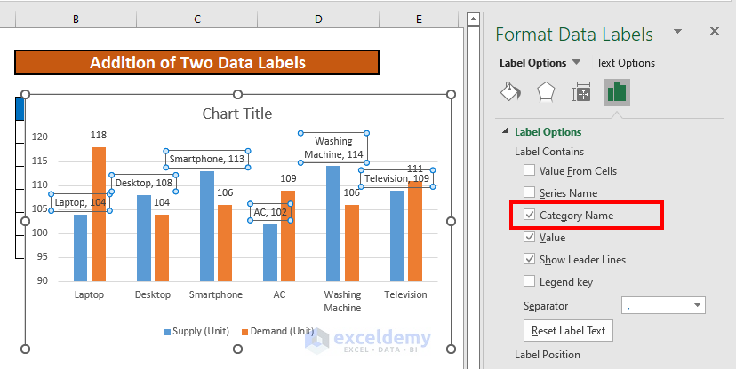
How to Add Two Data Labels in Excel Chart (with Easy Steps) 4 Quick Steps to Add Two Data Labels in Excel Chart Step 1: Create a Chart to Represent Data Step 2: Add 1st Data Label in Excel Chart Step 3: Apply 2nd Data Label in Excel Chart Step 4: Format Data Labels to Show Two Data Labels Things to Remember Conclusion Related Articles Download Practice Workbook How to Use Cell Values for Excel Chart Labels - How-To Geek Select the chart, choose the "Chart Elements" option, click the "Data Labels" arrow, and then "More Options.". Uncheck the "Value" box and check the "Value From Cells" box. Select cells C2:C6 to use for the data label range and then click the "OK" button. The values from these cells are now used for the chart data labels. Add data labels and callouts to charts in Excel 365 - EasyTweaks.com Step #2: When you select the "Add Labels" option, all the different portions of the chart will automatically take on the corresponding values in the table that you used to generate the chart. The values in your chat labels are dynamic and will automatically change when the source value in the table changes. Step #3: Format the data labels. Add or remove data labels in a chart - Microsoft Support Click the data series or chart. To label one data point, after clicking the series, click that data point. In the upper right corner, next to the chart, click Add Chart Element > Data Labels. To change the location, click the arrow, and choose an option. If you want to show your data label inside a text bubble shape, click Data Callout.
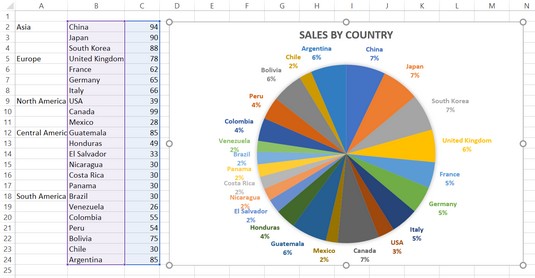
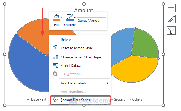
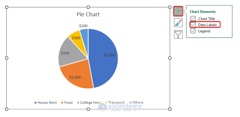
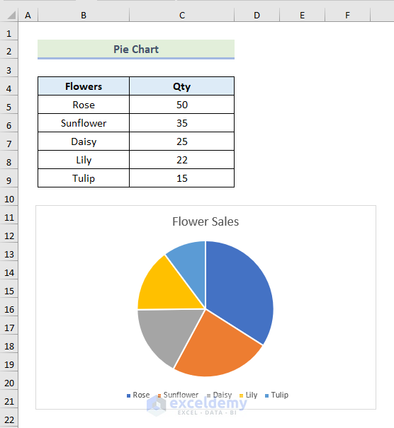
How to Make a Pie Chart with Multiple Data in Excel (2 Ways) - ExcelDemy First, to add Data Labels, click on the Plus sign as marked in the following picture. After that, check the box of Data Labels. At this stage, you will be able to see that all of your data has labels now. Next, right-click on any of the labels and select Format Data Labels. After that, a new dialogue box named Format Data Labels will pop up. How to Make Pie Chart with Labels both Inside and Outside Right click on the pie chart, click " Add Data Labels "; 2. Right click on the data label, click " Format Data Labels " in the dialog box; 3. In the " Format Data Labels " window, select " value ", " Show Leader Lines ", and then " Inside End " in the Label Position section; Step 10: Set second chart as Secondary Axis: 1. Change the format of data labels in a chart - Microsoft Support To get there, after adding your data labels, select the data label to format, and then click Chart Elements > Data Labels > More Options. To go to the appropriate area, click one of the four icons ( Fill & Line, Effects, Size & Properties ( Layout & Properties in Outlook or Word), or Label Options) shown here. Possible to add second data label to pie chart? - excelforum.com Re: Possible to add second data label to pie chart? Create the composite label in a worksheet column by concatenating the data in other cells and the nextline character, CHR (10). Now, use this composite label column as the source for Rob Bovey's add-in. -- Regards, Tushar Mehta Excel, PowerPoint, and VBA add-ins, tutorials
How to make a pie chart in Excel
Adding data labels to a pie chart - Excel General - OzGrid Free Excel ... Re: Adding data labels to a pie chart. Thanks again, norie. Really appreciate the help. I tried recording a macro while doing it manually (before my first post). But it didn't record anything about labels, much less making them bold.

How to Make Pie Chart with Labels both Inside and Outside ...
excel - Pie Chart VBA DataLabel Formatting - Stack Overflow Excel VBA to fill pie chart colors from cells with conditional formatting. 0. ... Formatting chart data labels with VBA. 1. Excel VBA Updating Chart Series. 0. Formatting charts in a chart group. ... Fastest decay of Fourier transform of function of (one-sided or two-sided) exponential decay ...

Best Excel Tutorial - Multi Level Pie Chart
How to Add Two Data Labels In Excel Chart? - YouTube In this video tutorial, we are going to learn, how to add multiple data labels in excel pie chart.Our YouTube Channels Travel Volg Channelhttps:// ...

How to suppress 0 values in an Excel chart | TechRepublic
2 data labels per bar? - Microsoft Community Use a formula to aggregate the information in a worksheet cell and then link the data label to the worksheet cell. See Data Labels Tushar Mehta (Technology and Operations Consulting) (Excel and PowerPoint add-ins and tutorials) Microsoft MVP Excel 2000-Present
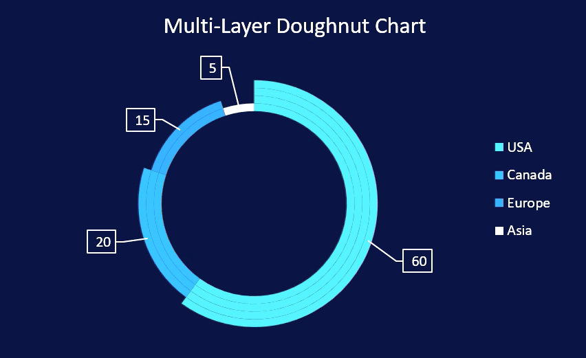
How to create a creative multi-layer Doughnut Chart in Excel
Creating Pie Chart and Adding/Formatting Data Labels (Excel) Creating Pie Chart and Adding/Formatting Data Labels (Excel) Creating Pie Chart and Adding/Formatting Data Labels (Excel)
Custom data labels in a chart
How to add two data labels for the same data on a pie chart?

How to Make a Pie Chart in Excel – Contextures Blog
Pie Chart in Excel | How to Create Pie Chart - EDUCBA Go to the Insert tab and click on a PIE. Step 2: once you click on a 2-D Pie chart, it will insert the blank chart as shown in the below image. Step 3: Right-click on the chart and choose Select Data. Step 4: once you click on Select Data, it will open the below box. Step 5: Now click on the Add button. it will open the below box.
5 New Charts to Visually Display Data in Excel 2019 - dummies
Microsoft Excel Tutorials: Add Data Labels to a Pie Chart - Home and Learn You should get the following menu: From the menu, select Add Data Labels. New data labels will then appear on your chart: The values are in percentages in Excel 2007, however. To change this, right click your chart again. From the menu, select Format Data Labels: When you click Format Data Labels , you should get a dialogue box. This one:

How to make a pie chart in Excel
How to add data labels from different column in an Excel chart? Right click the data series in the chart, and select Add Data Labels > Add Data Labels from the context menu to add data labels. 2. Click any data label to select all data labels, and then click the specified data label to select it only in the chart. 3.

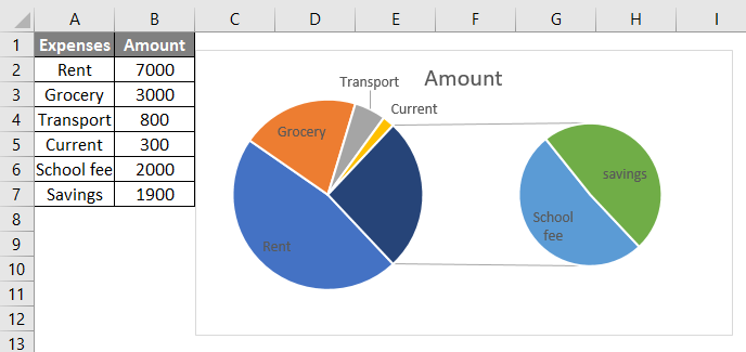
How to create pie of pie or bar of pie chart in Excel?
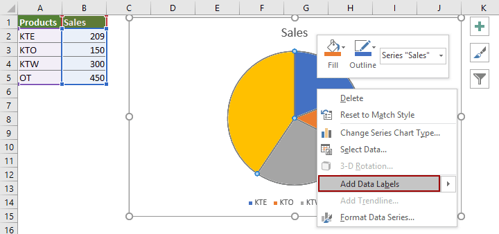
How to Create and Format a Pie Chart in Excel - Lifewire To add data labels to a pie chart: Select the plot area of the pie chart. Right-click the chart. Select Add Data Labels . Select Add Data Labels. In this example, the sales for each cookie is added to the slices of the pie chart. Change Colors

How to Make a Pie Chart in Excel
Create two data labels in pie chart? | MrExcel Message Board You have already figured out how to add an image that fills the sector of the pie chart but as far as I know you cannot add an icon or image over the actual pie chart sector, in such a way that it adjusts with the values. If you add it as a static image next to the legend, at least the legend does not move when the values change. Cheers.
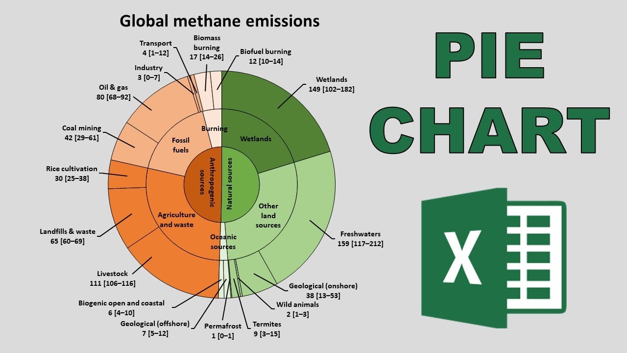
How to make a multilayer pie chart in Excel
Excel Pie Chart - How to Create & Customize? (Top 5 Types) Select the cell range A1:B7 > go to the " Insert " tab > go to the " Charts " group > click on the " Insert Pie or Doughnut Chart " drop-down > click the " Pie " type in the " 2-D Pie " option, as shown below. #Adding Data Labels We will customize the Pie Chart in Excel by Adding Data Labels.

How to Change Excel Chart Data Labels to Custom Values?
Multiple Data Labels on a Pie Chart | MrExcel Message Board So I have a table with 8 rows and 3 columns. This table includes: Column 1 - shipment name Column 2 - shipment cost Column 3 - shipment weight I have created a pie chart from this table, which covers the first two columns. Displayed next to each slice is a label with the shipment name, shipment cost, and percent share of the pie.

How to make a pie chart in Excel
How to Add Two Data Labels in Excel Chart (with Easy Steps ...

Microsoft Excel Tutorials: Add Data Labels to a Pie Chart

Presenting Data with Charts

Adding rich data labels to charts in Excel 2013 | Microsoft ...

How to make a pie chart in Excel
How to Make a Pie Chart with Multiple Data in Excel (2 Ways)

How to Create a Pie Chart in Excel | Smartsheet

vba - Excel Prevent overlapping of data labels in pie chart ...
How to Make a Pie Chart with Multiple Data in Excel (2 Ways)

Add or remove data labels in a chart - Microsoft Support
When to use Pie Charts in Dashboards - Best Practices | Excel ...

How to make a pie chart in Excel
Excel pie chart: How to combine smaller values in a single ...
How to Make Pie Chart with Labels both Inside and Outside ...
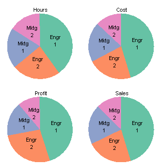
Column Chart to Replace Multiple Pie Charts - Peltier Tech
Presenting Data with Charts

Creating Pie Chart and Adding/Formatting Data Labels (Excel)

Add or remove data labels in a chart - Microsoft Support

Interactive R pie chart labels. Statistics for Ecologists ...
How to Make a Pie Chart with Multiple Data in Excel (2 Ways)

How to insert data labels to a Pie chart in Excel 2013

Change color of data label placed, using the 'best fit ...
How to make an Excel pie chart with percentages

How to Data Labels in a Pie chart in Excel 2010
Presenting Data with Charts
How to show percentage in pie chart in Excel?

Adding rich data labels to charts in Excel 2013 | Microsoft ...
How to Create a Pie Chart in Excel | Smartsheet

Excel charts: add title, customize chart axis, legend and ...

How to Make Pie Chart with Labels both Inside and Outside ...
Pie Chart Examples | Types of Pie Charts in Excel with Examples
Post a Comment for "45 how to add two data labels in excel pie chart"